Excel: Stock-out probability and Stock quantity | Supply Chain

Supply chain management often involves handling variability, especially when it comes to demand forecasting.
Let's explore an example that you can solve using Excel, helping you deal with challenges like fluctuating customer demand.

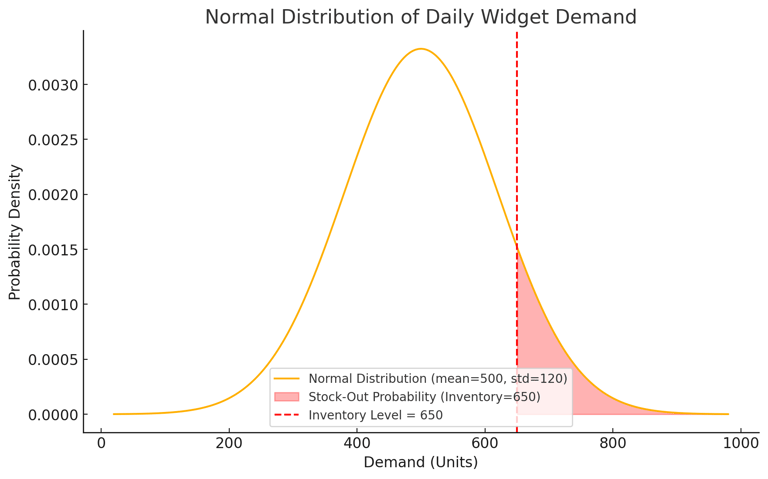
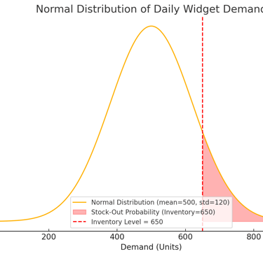
Imagine you're managing a warehouse that supplies widgets to a retailer. The daily demand for widgets is Normally distributed with a mean of 500 units and a standard deviation of 120 units.

Let's determine the Probability of Stock-out: Suppose you have 650 widgets in stock for a given day. What is the probability that the demand exceeds your inventory, meaning you will run out?

We can use Excel's =NORM.DIST function to solve this.

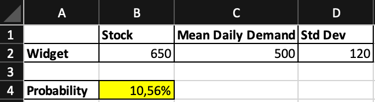
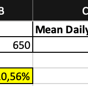
In Excel, enter the mean and standard deviation in cells C2 and D2, respectively, and enter your inventory level (650) in cell B2.

Use the formula: =1-NORM.DIST(B2; C2; D2; TRUE) This formula will give you the probability of running out, by calculating the area under the normal distribution curve beyond 650

We have a 10,56% of probability to stock-out, your supply chain can be concerning, depending on the nature of your business and the specific supply chain conditions

What if we want to ensure a 5% Stock-out risk? We want to prepare enough widgets to ensure only a 5% chance of running out on any given day. How many widgets should we stock?

We can use the =NORM.INV function for this.
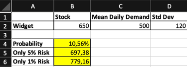
And use the formula: =NORM.INV(0,95; C2; D2) This function will give you the inventory level required to have only a 5% risk of running out. The 0.95 represents the 95th percentile, ensuring only a 5% chance of exceeding the stock.

Reducing the Stock-out Risk to 1% Now, you want to be even more confident that you won’t run out, targeting only a 1% probability of stock-out. How many widgets should you stock?
Again, use the NORM.INV function, but adjust the percentile.
Use the formula: =NORM.INV(0,99; C2; D2) This will give you the inventory level required to have only a 1% probability of running out, making your operations even more robust against variability.

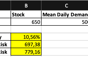
This are the results;

A stock-out directly translates to missed sales opportunities. Customers may switch to competitors, leading to lost revenue, which can be substantial, especially in a highly competitive market.
When stock-outs occur, you may need to expedite replenishment, which can increase costs through rush shipping or emergency procurement. Alternatively, you may lose sales altogether if customers choose not to wait.

We can lower and reduce the risk of stock-out simply by changing the percentile of the formula.

Here's the graph of the normal distribution for the daily widget demand. The bell curve represents the normal distribution with a mean of 500 units and a standard deviation of 120 units.
The shaded red area to the right of the inventory level of 650 represents the probability of a stock-out, indicating the chance that demand will exceed your available inventory.

Lowering stock-out probability to 5% or 1% is crucial for maintaining customer satisfaction, ensuring steady revenue, and protecting your brand reputation. Frequent stock-outs can lead to lost sales as customers turn to competitors, damage to your brand’s image, and increased operational costs from emergency restocking efforts. A low stock-out probability fosters stronger customer loyalty by ensuring products are consistently available, which is critical in competitive markets. Additionally, reducing stock-out risks enhances supply chain resilience, allowing you to respond better to demand fluctuations and unexpected disruptions. Ultimately, it boosts your market position and long-term growth potential by ensuring reliability and operational efficiency.

In supply chain management, a normal distribution is often applicable when we deal with situations involving natural variability, where data tends to cluster around a central value with symmetric deviations.

While the normal distribution is widely applicable, there are situations where it may not be the best fit:

• Highly Skewed Demand: When the majority of demand happens during special occasions like holidays, the normal distribution won't accurately represent the data. Instead, you might use a Poisson distribution for rare events or an exponential distribution for processes with time dependencies.

• New Product Introductions: Demand might have heavy tailed distributions or may follow irregular patterns. In such cases, normal distribution is unsuitable because there’s not enough historical data or the variability is too great.

• Intermittent Demand: Products that experience this, such as spare parts, will not have a normal distribution. Instead, a discrete distribution such as Poisson or negative binomial may be used to better model infrequent demand spikes.
  

We will see all these cases, in future practical examples.